Contents

This document is a draft, with some terminology yet to be defined/updated.

Density Estimation using Gaussian Process

Introduction

Since its inception in the late-17th century by Robert Hooke, schlieren has been used in the sciences, engineering and even the arts. The types of flows captured have been diverse, ranging from the shock waves of an aircraft and the mixing of turbulent jets to plumes over a candle, and even the dissolution of particles in a solution. Scientifically, these images have shaped our understanding of fluid mechanics, whilst more generally, they have and continue to inspire curiosity in the natural world. The schlieren method relies on the behaviour of light when passing through different mediums. Light either slows down or refracts depending on the homogeneous nature of the medium. When encountering a homogeneous medium, the light rays will pass through uniformly, but if the light rays pass through regions of inhomogeneity, they will refract in proportion to the gradient of the refractive index of the inhomogeneities [1, 2].

The advantage of a schlieren image lies in the fact that the refractive index is dependent on the density of the medium it passes through. Knowledge of this relationship is one of the steps that allows us to obtain quantitative data from such images. Let \(\rho \left( x, y \right)\) be the spatially varying density of a fluid surrounding an object of interest; it is expressed as a scalar-field with a horizontal coordinate \(x\) and a vertical coordinate \(y\). It has a linear relationship with the refractive index \(n \left(x, y \right)\), given by

(1)\[ n\left( x, y \right) - 1 = \kappa \rho \left( x, y \right) \label{equ:gdale} \]

where \(\kappa\) is the Gladstone-Dale coefficient. A schlieren image represents the refractive index gradient field \(\nabla n\), where the gradient direction is based on the orientation of the knife edge: placement in the vertical direction yields \(\partial n / \partial x\), whilst placement along the horizontal direction renders \(\partial n / \partial y\) [3].

Pixels to Density via Machine Learning

Our approach to schlieren imaging in this paper takes a decidedly alternate route from the prior quantitative efforts referenced above. We leverage ideas from machine learning, namely Gaussian process regression [4], to facilitate the spatial estimation of density. To set the stage, we begin by defining a few quantities. Let \(\rho \left( x, y \right)\) be the spatially varying density field, \(\partial \tilde{\rho}\left( x, y \right) / \partial x\) be the schlieren image, taken with a vertical knife-edge, and \(\partial \tilde{\rho}\left( x, y \right) / \partial y\) be the schlieren image, taken with a horizontal knife-edge.

Gaussian processes

A Gaussian process is a spatially varying function, which at any spatial location admits a Gaussian distribution. As our focus will be on bivariate functions, we introduce a Gaussian process as

(2)\[ f\left( x, y \right) \sim \mathcal{N}\left[ \boldsymbol{\mu} \left( x, y \right), \mathbf{C} \left( x, y, x', y' \right) \right] \]

which is entirely defined by its mean \(\boldsymbol{\mu}\) and covariance \(\mathbf{C}\) functions. The covariance function tries to imbue a spatial relationship across spatial locations and is set by a kernel function \(k\left( \cdot, \cdot \right)\), where the two arguments correspond to two different spatial locations. Standard choices for the kernel function include linear, squared exponential, and Mat’{e}rn to name a few (see Chapter 4 in [4] for more). These and others can be tuned to characterise some of the physics-driven phenomenon that defines how the value of some quantity of interest will varying from location to location. Kernel functions in turn are parameterised by certain hyperparameters, whose values are typically the outcome of an optimisation—via maximum likelihood estimation or cross validation—or extensive sampling procedure—via Markov chain Monte Carlo (MCMC) as elucidated further below.

From a regression context, the problem is to determine (2) given observations \(\left\{ (x^{\ast}_i, y^{\ast}_i), f_i \right\}_{i=1}^{N}\), where \(\left(x^{\ast}_i, y^{\ast}_i \right)\) are the input spatial coordinates at which output function values \(f^{\ast}_i\) are observed. Further, one typically assumes that each output function value is corrupted by a small observational or sensor noise \(\left\{\varepsilon_i \right\}_{i=1}^{N}\), where for simplicity we assume that \(\varepsilon \sim \mathcal{N}\left(0, \sigma_y^2 \right)\). This data can be used to define a joint distribution

(3)\[\begin{split} \left(\begin{array}{c} f^{\ast}\\ f \end{array}\right)=\left[\left(\begin{array}{c} \boldsymbol{0}\\ \boldsymbol{0} \end{array}\right),\left(\begin{array}{cc} \mathbf{K}_{\ast\ast}+ \boldsymbol{\Sigma} & \mathbf{K}_{\ast}\\ \mathbf{K}_{\ast}^{T} & \mathbf{K} \end{array}\right)\right], \end{split}\]

where the \(i,j\) entries of the kernel matrices is given by

(4)\[\begin{equation} \left[ \mathbf{K}_{\ast \ast} \right]_{ij} = k \left( \left(x_{i}^{\ast}, y_{i}^{\ast} \right) , \left(x_{j}^{\ast}, y_{j}^{\ast} \right)' \right) \end{equation}\]

(5)\[\begin{equation} \left[ \mathbf{K}_{\ast} \right]_{ij} = k \left( \left(x_{i}^{\ast}, y_{i}^{\ast} \right) , \left(x_{j}, y_{j} \right)' \right), \end{equation}\]

and

(6)\[\begin{equation} \left[ \mathbf{K} \right]_{ij} = k \left( \left(x_{i}, y_{i} \right) , \left(x_{j}, y_{j} \right)' \right). \end{equation}\]

In (3), \(\boldsymbol{\Sigma}\) corresponds to the noise matrix, which we assume to be \(\boldsymbol{\Sigma} = \sigma_y^2 I\), where \(I\) is the \(N \times N\) identity matrix. Expressions for the mean and covariance of \(f\) at any \(\left(x, y \right)\) conditioned upon the input-output data pairs is then written as

(7)\[\begin{eqnarray} \boldsymbol{\mu} \left( x, y \right) | \left\{ (x^{\ast}_i, y^{\ast}_i), f^{\ast}_i \right\}_{i=1}^{N} = && \mathbf{K}_{\ast}^{T} \left(\mathbf{K}_{\ast \ast} + \boldsymbol{\Sigma} \right)^{-1} \left( f^{\ast}_1, \ldots, f^{\ast}_N \right)^{T}, \end{eqnarray}\]

(8)\[\begin{eqnarray} \mathbf{C} \left( x, y \right) | \left\{ (x^{\ast}_i, y^{\ast}_i), f^{\ast}_i \right\}_{i=1}^{N} = && \mathbf{K} - \mathbf{K}_{\ast}^{T} \left(\mathbf{K}_{\ast \ast} + \boldsymbol{\Sigma} \right)^{-1} \mathbf{K}_{\ast}. \end{eqnarray}\]

which are standard expressions, as found in [4].

Gaussian process regression can be interpreted as the maximisation of the probability of observing the (noisy) data, given certain structural assumptions encoded into the kernel function \(k\) about the data. Infact, within a Bayesian context, these concepts are referred to as the likelihood and the prior respectively. This view can be more rigorously formulated into an optimisation problem, where one seeks to identify the hyperparameters that maximize the marginal likelihood. Certain modifications need to be made to the joint distribution in light of the physical nature of the schlieren data observed.

From schlieren to density

This subsection describes the changes needed to the joint distribution to account for the schlieren image inputs. Let \(\left\{ (x^{\ast}_i, y^{\ast}_i)\right\}_{i=1}^{N}\) denote the horizontal and vertical locations of \(N\) pixels in a schlieren image. Let \(s^{\ast} \in \left[0, 255 \right]\) be the intensity values at these \(N\) pixels. From the Gladstone-Dale expression (1), we can define the linear relationship between the density gradient and the refractive index gradient field captured by the schlieren apparatus

(9)\[\begin{equation} s_x = \alpha_x \frac{\partial \rho}{\partial x} + \beta_x, \end{equation}\]

(10)\[\begin{equation} s_y = \alpha_y \frac{\partial \rho}{\partial y} + \beta_y \end{equation}\]

We define another joint distribution, which is also Gaussian, by applying the linear differential operator \(\partial \left( \cdot \right)\) on (3), yielding

(11)\[\begin{split} \left(\begin{array}{c} s^{\ast}_x\\ s^{\ast}_y\\ f \end{array}\right)=\left[\left(\begin{array}{c} -\beta_x\\ -\beta_y\\ \boldsymbol{0} \end{array}\right),\left(\begin{array}{ccc} \alpha_x^2 \partial_x^2 K_{\ast\ast} & \alpha_x \alpha_y \partial_{xy} K_{\ast\ast} & \alpha_x \partial K_{\ast x} \\ \alpha_y \alpha_x \partial_{yx} K_{\ast\ast} & \alpha_y^2 \partial_{y}^2 K_{\ast\ast} & \alpha_y \partial K_{\ast y} \\ (\alpha_x \partial K_{\ast x})^{T} & (\alpha_y \partial K_{\ast y})^{T} & K % v_1& % v_2& % v_3 \end{array}\right)\right], \end{split}\]

where the \(i,j\) entries of the kernel matrices is given by

(12)\[\begin{align} \left[ \partial^2 K_{\ast \ast} \right]_{ij} &= \frac{\partial^2 k}{\partial ^2 } \left( \left(x_{i}^{\ast}, y_{i}^{\ast} \right) , \left(x_{j}^{\ast}, y_{j}^{\ast} \right)' \right), \nonumber \\ \left[ \partial K_{\ast} \right]_{ij} &= \frac{\partial k}{\partial } \left( \left(x_{i}^{\ast}, y_{i}^{\ast} \right) , \left(x_{j}, y_{j} \right)' \right). \end{align}\]

from which the density \(\rho\) can be written by

(13)\[ \rho \left(x, y \right) \sim \mathcal{N} \left( \boldsymbol{\mu}_{\rho}\left(x, y \right), C_{\rho}\left(x, y \right) \right), \]

where

(14)\[ \boldsymbol{\mu}_{\rho} \left( x, y \right) | \left\{ (x^{\ast}_i, y^{\ast}_i), s^{\ast}_i \right\}_{i=1}^{N} = \partial K_{\ast}^{T} \left(\partial^2K_{\ast \ast} + \boldsymbol{\Sigma} \right)^{-1} \times \left( s^{\ast}_1, \ldots, s^{\ast}_N, f_1, \ldots, f_N \right)^{T}, \]

(15)\[\begin{eqnarray} C_{\rho} \left( x, y \right) | \left\{ (x^{\ast}_i, y^{\ast}_i), s^{\ast}_i \right\}_{i=1}^{N} = && K - \partial K_{\ast}^{T} \left( \partial^2 K_{\ast \ast} + \boldsymbol{\Sigma} \right)^{-1} \partial K_{\ast}. \end{eqnarray}\]

Note that in constructing (13) we have effectively estimated \(\rho\) from observations of \(\partial \tilde{\rho} / \partial x\) and \(\partial \tilde{\rho} / \partial y\).

A few additional comments are in order here. First, although the noise matrix \(\boldsymbol{\Sigma}\) was defined to be diagonal, it need not be and correlations can be imposed. Furthermore, \(\boldsymbol{\Sigma}\) can have different variances, depending on the corresponding pixel values in \(f\). There is some rationale behind such a proposal: given that pixel values in schlieren images are cropped to fall within \([0, 255]\), regions that have very low, or very high refractive gradients will likely look similar. Thus, there will be greater uncertainty in the pixel values in such regions, compared to others.

Second, from the block matrices in (11), it should be readily apparent that we are limited to twice differentiable kernel functions \(k\). Throughout this paper we adopt the squared exponential kernel, which in two dimensions is given by

(16)\[\begin{equation} k \left( \left(x , y \right) , \left(x , y \right)'; \sigma_f, l_x, l_y \right) = \sigma_f^2 \ \textrm{exp} \left( p \right), \end{equation}\]

where,

\[\begin{equation*} p = \frac{1}{2} \left[ \frac{\left(x - x' \right)^2}{l_x^2} + \frac{\left(y - y' \right)^2}{l_y^2} \right]. \end{equation*}\]

where \(\boldsymbol{\theta} = \left( \sigma_f, l_x, l_y, \alpha_x, \alpha_y, \beta_x, \beta_y \right)\) are the tunable hyperparameters, which control the signal variance and the length scales respectively. As alluded to before, suitable values of the hyperparameters can be obtained by solving an optimisation problem.

A subset of the joint distribution defined in (11) can be used if an image is available for only one gradient direction with the caveat that the posterior mean will not fully represent the density field unless the flow is highly directional and the gradient in the other direction is negligible. The joint distribution for a case where \(s^{\ast}_x = \partial \tilde{\rho}/\partial x\) is available would be

(17)\[\begin{split} \left(\begin{array}{c} s^{\ast}_x\\ f \end{array}\right)=\left[\left(\begin{array}{c} -\beta_x\\ \boldsymbol{0} \end{array}\right),\left(\begin{array}{ccc} \alpha_x^2 \partial_x^2 K_{\ast\ast} & \alpha_x \partial K_{\ast x} \\ (\alpha_x \partial K_{\ast x})^{T} & K \end{array}\right)\right] \end{split}\]

with \((.)_x\) replaced by \((.)_y\) if \(s^{\ast}_y = \partial \tilde{\rho}/\partial y\) is available instead.

Results

Analytical case

A simple analytical function is used to define a model density field and its corresponding density gradient. The density gradients are normalised to pixel values (\(s^{\ast} \in \left[0, 255 \right]\)) to emulate a Schlieren image with an unknown range, and a random sampling of 200 are selected from this image for use as observation data (white circles in Figure 1), with three random density sampling locations also used (green circles in Figure 1). The density and its partial derivative w.r.t \(x\) and \(y\) for this case are given as

(18)\[\begin{split} \begin{split} \rho &= sin( x^2 ) (2y - 3)/10 + 1.5, \\ \frac{\partial{\rho}}{\partial{x}} &= x\ cos(x^2) (2y - 3)/5, \\ \frac{\partial{\rho}}{\partial{y}} &= sin(x^2)/5. \end{split} \ \end{split}\]

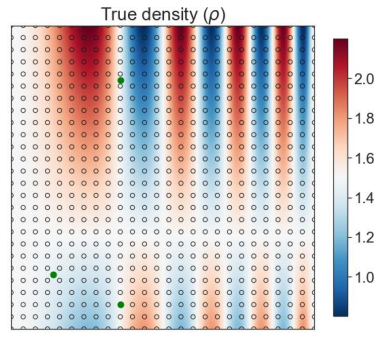
Fig. 1 Analytical test case sampling locations.

Figure 2 showing a comparison of the true density (a) against the posterior predicted mean density (d), and the corresponding prediction of the gradients (e-f), and the posterior standard deviation shown in (g) exhibiting a generally uniform and small standard deviation demonstrates a high level of model confidence.

More details regarding the set-up required will be published in a paper soon.

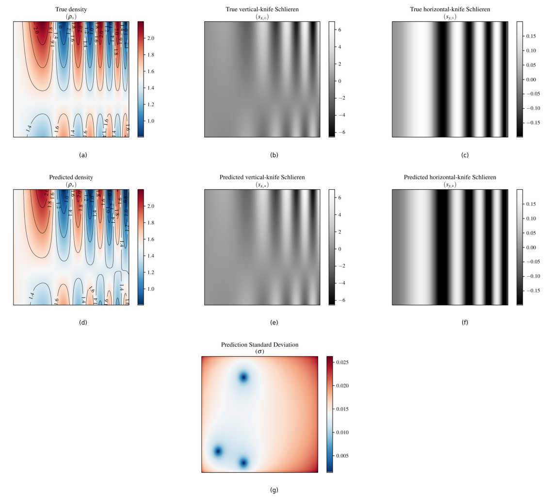
Fig. 2 Analytical test case: (a) true density (\(\rho\)); (b) true vertical knife edge Schlieren image; (c) true horizontal knife edge Schlieren image; (d) GP predicted density; (e) GP predicted vertical knife edge Schlieren image; (f) GP predicted horizontal knife edge Schlieren image; (g) posterior standard deviation.

Wind tunnel sting model

Consider the asymmetrical sting model in supersonic flow (\(M_\infty =\) 2.0) published by Ota et al. [5]. The reconstructed density published in that paper, using BOS, is assumed to be representative of the true density, and thus serves as our benchmark for comparison. Figure 3 captures the experimental results with the vertical knife-edge schlieren image in (a); horizontal knife-edge schlieren image in (b), and the BOS yielded density reconstruction in (c). Note that for subfigures (a) and (b) the colours denote greyscale pixel values between \([0,255]\), whilst the colours in (c) represent the density in units of \(kg/m^3\). Another point to note is that only the upper half of the schlieren images are used for this reconstruction, as the shock captured across the lower half sees excessive clipping.

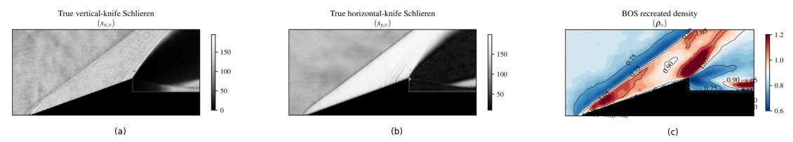
Fig. 3 Experimental schlieren results from Ota et al. [5]: (a) vertical knife-edge schlieren image; (b) horizontal knife-edge schlieren image, and (c) BOS yielded density estimation.

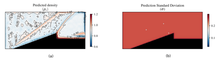
Fig. 4 Experimental schlieren results from Heineck et al. [6, 7]: (a) vertical knife-edge schlieren image, and (b) horizontal knife-edge schlieren image. Our estimate of some of the flow quantities in (c) and the uncertainties therein.

The reconstructed density is shown in Figure 4 with the mean in (a) and the standard deviation in (b). The mean follows the expected trend of a uniform density upstream of the shock followed by a rapid increase in density across the shock, before decreasing across the expansion fan. Due to clipping of the input schlieren images, the gradients in region downstream of the expansion fan are not captured (the gradients are close to zero), hence this is represented as the mean of the observed densities instead.

The BOS density in subplot Figure 3 (c) does not follow the expected behaviour of oblique shocks in theory, where, the density upstream of the shock must be uniform with a sharp increase in density across the shock. This may be caused by optical distortion incurred when performing BOS. Additionally, the shock itself should be captured as a very thin band, which is what is captured in our reconstruction, along with the shear layer downstream.

Supersonic aircraft in flight

Next, we study schlieren images taken by NASA of a T-38 training jet at a Mach number of 1.05. The horizontal and vertical knife-edge schlieren images captured in [6, 7] are shown in Figure 5 (a) and (b) respectively. Additionally, based on estimates of the ambient conditions of the flight and estimates of shock and wedge angles, we can estimate the density at three points as shown in Figure 5(c). The two freestream points are assigned the same value of density, whilst the density at the third (remaining) point is estimated via standard shock relations.

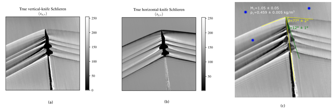
Fig. 5 Experimental schlieren results from Heineck et al. [6, 7]: (a) vertical knife-edge schlieren image, and (b) horizontal knife-edge schlieren image. Our estimate of some of the flow quantities in (c) and the uncertainties therein.

As true density fields are not available for this case, and at least one known density is required from a non-freestream region for this method, the density after the first oblique shock wave is estimated. Two quantities are used to calculate the density: (i) the known experimental altitude of 30,000 ft and thus the freestream density; (ii) the standdard shock relations, accounting for uncertainties in the Mach number and angles. However, note that this is a simplification, as the wedge angle calculation does not account for the three-dimensional relief effect. This density data, along with horizontal and vertical knife-edge schlieren images are sub-sampled (to reduce the computational overhead), and fed into the machine learning workflow. For the inputs to the GP, the aircraft region is masked out, as it is the geometry and is not part of the flow.

The predicted density and standard deviation are shown in Figure Figure 6, with each shock clearly visible in the prediction.

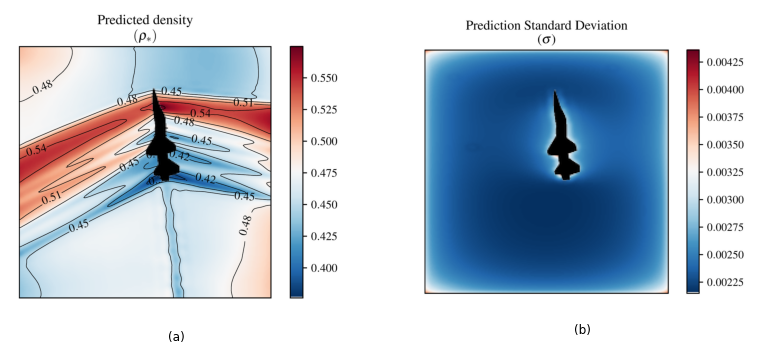
Fig. 6 Density reconstruction from the vertical and horizontal knife-edge schlieren images of the supersonic aircraft, obtained as a Gaussian process with (a) mean; (b) standard deviation. Both are moments with units of \(kg/m^3\).

Shock tube CFD

In this section, we consider a canonical Sod shock tube\cite{Sod1978} test case. The CFD simulation result provided by Dzanic and Witherden [8] is used, with the full primitive flow variables available for comparison. Figure 7 shows a set of results from one timestep that are used as inputs to the GP. To simulate a schlieren image, the density gradient is calculated, and normalised to standard pixel value range of between 0 and 255. Figure 7 shows the vertical knife-edge schlieren result in (a); horizontal knife-edge schlieren image in (b), and the true density obtained by CFD (c).

Fig. 7 Numerical results of shock tube test case [8]: (a) vertical knife-edge schlieren image; (b) horizontal knife-edge schlieren image, and (c) True density from CFD.

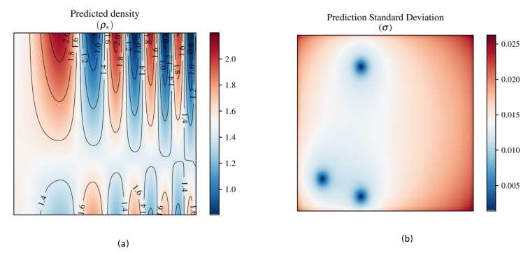
Fig. 8 Density reconstruction from the vertical and horizontal knife-edge schlieren images of the shocktube case, obtained as a Gaussian process with (a) mean; (b) standard deviation. Both are moments with units of \(kg/m^3\).

References

1

J. Rienitz. Schlieren experiment 300 years ago. Nature 1975 254:5498, 254:293–295, 1975. URL: https://www.nature.com/articles/254293a0, doi:10.1038/254293a0.

2

G. S. Settles. Schlieren and Shadowgraph Techniques. Springer Berlin Heidelberg, 2001. doi:10.1007/978-3-642-56640-0.

3

Michael J Hargather and Gary S Settles. A comparison of three quantitative schlieren techniques. Optics and Lasers in Engineering, 50(1):8–17, 2012.

4(1,2,3)

Carl Edward Rasmussen and Christopher KI Williams. Gaussian Processes for Machine Learning. Adaptive Computation and Machine Learning. MIT Press, Cambridge, MA, USA, January 2006.

5(1,2)

Masanori Ota, Kenta Hamada, Hiroko Kato, and Kazuo Maeno. Computed-tomographic density measurement of supersonic flow field by colored-grid background oriented schlieren (CGBOS) technique. Measurement Science and Technology, 22(10):104011, sep 2011. URL: https://doi.org/10.1088%2F0957-0233%2F22%2F10%2F104011, doi:10.1088/0957-0233/22/10/104011.

6(1,2,3)

James T. Heineck, Daniel W. Banks, Edward T. Schairer, Edward A. Haering, and Paul S. Bean. Background oriented schlieren (BOS) of a supersonic aircraft in flight. In AIAA Flight Testing Conference, number June. 2016. doi:10.2514/6.2016-3356.

7(1,2,3)

James T. Heineck, Daniel W. Banks, Nathanial T. Smith, Edward T. Schairer, Paul S. Bean, and Troy Robillos. Background-oriented schlieren imaging of supersonic aircraft in flight. AIAA Journal, 59:11–21, 9 2021. URL: https://arc.aiaa.org/doi/abs/10.2514/1.J059495, doi:10.2514/1.J059495.

8(1,2)

Tarik Dzanic and Freddie D. Witherden. Positivity-preserving entropy-based adaptive filtering for discontinuous spectral element methods. 1 2022. URL: https://arxiv.org/abs/2201.10502v2, doi:10.48550/arxiv.2201.10502.